How to merge cells in Google Sheets
Any data you enter into Google sheets is contained within a cell. There will be occasions when you want data from one cell to be stretched across a selection of cells. To do this you need to merge cells in Google Sheets.
Not always, but the majority of times merging cells is done to make a spreadsheet more presentable. I'll show you some examples of when you may want to merge cells. Then I'll show you the different ways you can merge cells in Google Sheets.
An example of when you might want to merge cells
Below you'll see a list of managers who are on a rota to work a particular shift. You'll notice that most of the cells contain data. However, you'll also notice the cell to the right of each day is empty. It's empty because no data is needed for this cell.
Although this is perfectly fine and works as it is. It would be clearer and more pleasing to the eye if the days of the week shown were centred between the two cells.
To make it easier to read and visually appealing the best option in this scenario would be to merge the cells. Once you've merged the cells, the merged cells act as one cell. You can then centre align that cell, as you can see below.
By merging the cells for the days of the week you can see it's much clearer to notice, which cells below are related to that day.
How to merge cells in Google Sheets
There are two ways you can merge cells in Google Sheets and both ways work exactly the same. The first way is to use the icon that is readily available from the main screen.
First, you need to select the range of cells that you wish to merge. In this example that would be cells A1 and B1. Cell A1 contains 'Monday' and cell B2 is empty. Simply select this range with your mouse or keyboard.
Cells A1 and B1 have been highlighted
Once you've selected the range of cells by highlighting them, as shown above. You simply need to click on the merge cells icon, as shown below.
Click on the merge cell icon
Once you've done this you'll notice cells A1 and B1 have been merged together. Merging the cells together may not make much of a difference visually at first. You'll most likely want to centre align the cells to make the day of the week centre between cells A1 and B1.
Once the cells have been merged you may want to centre align as shown above
Once you've centred aligned the merged cells you'll notice the data in the first cell (A1). Is now centred between cells A1 and B2.
How to merge cells in Google Sheets
Another way to merge cells
The following method works exactly the same. The only difference is how you merge the cells. Instead of using the icon from the main page. You can also choose to merge cells from a drop-down menu. Again, you need to highlight the range of cells you wish to merge.
Once you've highlighted the cells you wish to merge. You can merge the cells from the Format drop-down menu, as shown below.
Choose the merge cells option from the format drop-down menu
You can merge cells vertically or horizontally
You can merge cells in Google Sheets either vertically, horizontally or both at the same time. There may be times when you wish to do this. You can only merge cells that are directly adjacent to each other. Once you've merged a selection of cells they act as one.
If you wish to remove the merging of cells in Google Sheets. You simply select the merged cell and click on the merge cell icon. The cells will be unmerged and act as they did before any merging took place.
How to add or change the currency in Google Sheets
Many people use spreadsheets to record financial transactions. When entering numbers into a spreadsheet, by default, you'll not see a currency. Instead, the numbers are entered without any association to a specific currency.
In this article, you'll find out how to add a currency to a range of cells. You'll also find out how to change the default currency that is used.
When you want to change the properties of data entered into a spreadsheet. You need to remember that you're only changing the properties for the cells you've selected.
HOW TO USE CURRENCY OR CHANGE THE DEFAULT CURRENCY IN GOOGLE SHEETS
Time needed: 2 minutes.
This guide will show you how to add currency to a set of cells in Google Sheets. It will also show you how to change the default currency that is used.
Highlight the selected cellsYou need to highlight the selected cells where you want to add or change the currency.
Choose the Format menu in Google SheetsWhilst you have the cells highlighted use the mouse to click on the format menu at the top of your screen.
Choose the Number sub menuFrom the format menu, you want to choose the Number menu. You can do this by hovering or left-clicking with your mouse.
Change your selected cells to a currencyThe 'number' menu gives you the option to change the selected cells to a currency. Choosing this option will change the numbers in your selected cells to show the currency symbol in each cell. You'll notice the currency will default to your local currency.
Below you can see it has defaulted to British Pound Sterling.
Change the cells to show a rounded currencyThe above step will change your numbers to the selected currency. It will also show the first two numbers to the right of the decimal place. If you only want to show rounded numbers, you can do this by clicking on the 'Currency (rounded)' option.
Change to another currencyIf you want to use a currency other than the default currency, you can do this from the same menu. Click on the format menu and then hover over the 'number' submenu FORMAT>NUMBER and choose 'More Formats' from the bottom of the menu.
Choose more currenciesOnce you've clicked on 'More Formats' choose 'More Currencies' from the submenu as shown below.
Choose from the list of currenciesYou'll then be presented with a dialogue box, which shows a list of currencies. You can scroll up or down the list to find the currency. However, you can quickly find the currency by typing it into the search box at the top, as shown below.
You should now be able to easily change numbers in Google Sheets to a currency value. You've also learned how to change the default currency in Google Sheets.
How to add or remove decimal places in Google Sheets
When you open a new spreadsheet in Google Sheets, you'll notice the numbers are formatted in a particular way. This is fine if you're working on a basic spreadsheet and you want some quick results. However, there will be a time when you need to format the numbers to suit your project.
This article looks at all the different ways you can format numbers in Google Sheets. Most of the changes are pretty easy to do because Google Sheets comes with clickable icons that will do exactly what is needed.
DEFAULT FORMAT OF NUMBERS IN GOOGLE SHEETS
By default, you'll notice Google Sheets works with numbers in a specific way. In the example below I've entered five different numbers over five separate cells. You'll notice some have two decimal points and others have none.
However, when I entered these numbers, I used decimal points in all of the cells. Google Sheets, by default, only shows decimal places where it's necessary. If the figure is a whole number no decimal places are used. This is fine because there is no value in showing decimal places that contain a zero amount.
You may, however, decide this does not look very appealing and may even cause some confusion. To fix this you need to format the numbers in the cells to show decimal places for all numbers whether rounded or not.
HOW TO ADD OR REMOVE DECIMAL PLACES IN GOOGLE SHEETS
It's really quick and simple to add or remove decimal places in Google Sheets.
Time needed: 1 minute.
How to change the number of decimal points used in Google Sheets
Highlight the range of cells - First, you need to highlight the range of cells that you would like to format.
Click on the icon showing the two decimal places from the toolbar - On the default toolbar above your spreadsheet, you'll find the icon that adds decimal points to the range of cells you've currently highlighted. You'll notice the decimal places have now been used on the selected range of cells.
How to remove decimal places - If you wish to remove decimal places, you simply click on the icon shown below. This will remove a decimal place one at a time. Using both of these icons will allow you to set the exact number of decimal places you wish to use.
How to do a vlookup in Google Sheets
One of the most popular and powerful options in Google Sheets is the vlookup function. This powerful yet simple function allows you to do so much when using a spreadsheet.
Learning how to do a vlookup may appear difficult at first. However, once you have got used to how it works you will have no problem adding the vlookup function to your Google Sheets spreadsheet.
WHAT IS A VLOOKUP
A vlookup is a function that you will find in all spreadsheet programs. The vlookup function in Google Sheets works the same as it would in Microsoft Excel.
The purpose of a vlookup is to use specific criteria, which is stored in a cell to find other data within the spreadsheet that is linked to that criteria. It's a really quick way of getting information and it can be used for many different purposes.
This is one of the reasons why the vlookup is one of the most popular and loved functions in spreadsheets.
WHY A VLOOKUP IS USEFUL
A vlookup is useful when you have large amounts of data that you want to extract information from. Generally speaking you would have the raw data in a separate sheet. You would then add an extra sheet where you would use the vlookup function to extract the data from the sheet containing the raw data.
Let's take a look at how to do a basic vlookup in Google Sheets. In this example you own a business selling sports equipment. You want to setup a spreadsheet to record sales. To avoid having to enter all the information about the product every time you sell an item. You have decided to do a vlookup.
The vlookup will allow you to record sales by entering just one piece of information. In this example that is the 'product code' of the item, you have sold.
WATCH THE VIDEO
Below you'll find a full how-to guide on how to do a vlookup in Google Sheets. However, if you're a visual learner, I've created a video, which also goes into great detail on how to do a vlookup using Google Sheets.
HOW TO DO A VLOOKUP IN GOOGLE SHEETS
When using a vlookup you will usually have a large amount of raw data that you want to extract data from. It's always best to separate the raw data by adding an extra tab to your spreadsheet. Below you can see I have two tabs. One is called 'RAW_DATA' and the other 'vlookup'.
I have entered some basic raw data into the RAW_DATA tab. In this example, the raw data is the stock you have in your warehouse that is for sale. The information provides basic information about the product, which includes the product name, price, colour and stock levels.
I have then added the field names for the information I want to record when a sale takes place. This information has been added to the vlookup tab, as you can see below.
If you were not using a vlookup you would need to manually enter the information every time you sold an item. By doing a vlookup you will only need to enter the product code.
ENTERING THE VLOOKUP FORMULA IN GOOGLE SHEETS
We need to enter a vlookup formula in columns B to G. Column A is where you would manually type the product code.
Time needed: 6 minutes.
Entering the vlookup formula in cell B2
Select cell B2click on cell B2 with your mouse.
Start the vlookup formulaTo start a formula enter the '=' sign followed by vlookup without any spaces. =vlookup
Select the cell containing the product codeContinuing with your formula enter ( andclick on cell A2 with your mouse.
Select the raw dataSelect the 'Raw_Data' tab with your mouse. Then highlight the range of data needed for the vlookup. Do this by holding down your left mouse button on cell A2 and dragging your mouse to E14. Then release the mouse button.
Select the column you want to lookup from the raw dataYou now need to choose the column that contains the correct result. Do this by entering a comma and typing the column number, which is column number 2.
Close the vlookup formulaClose the vlookup by entering a comma and the word false. Then close with a bracket and press return.
You should now see the following in cell B2
You can see from above that the information is not yet showing. The reason for this is because we have not yet entered any information in cell A2. The formula needs information in cell A2 to find matching information in the Raw Data sheet.
Enter a product code in cell A2
Enter the product code BD401 in cell A2. Providing you have done the formula correctly you should now see something similar to what is showing below.
As you can see by entering the product code in cell A2. It has found matching information that matches the criteria of your vlookup formula.
UNDERSTANDING THE VLOOKUP FORMULA
So we have just entered the first vlookup needed for our sales spreadsheet. However, you may have questions about how the formula works. Before we go onto entering the remaining formulas let's take a look at each aspect of the vlookup, so you can get better understanding.
=vlookup(
This is what you enter to start the vlookup. Whenever you do a formula in Google Sheets you start with the '=' sign. You then need to tell Google Sheets what function to use, which you do by entering 'vlookup'.
To start selecting the criteria you open the formula with the open bracket '('.
=vlookup(a2,
You then need to select the column that contains data that matches data in your raw data. We have chosen the product code, which is in column A of your vlookup tab.
=vlookup(a2,RAW_DATA!A2:E14,
The next section of the vlookup is where you select the raw data. In our example we did this by clicking the 'RAW_DATA' tab and dragging the mouse over the cells containing the data.
As you can see from above when you do this it adds 'RAW_DATA!A2:E14 to the formula. This part of the formula is confirming the range of cells where the raw data is stored. It's also confirming this raw data is in the tab named 'RAW_DATA'.
When you become more familiar with vlookups in Google Sheets. You can just enter the formula by typing it in whole; rather than using your mouse to select the different sections. Either way works and it all depends on the vlookup and raw data you are working with.
=vlookup(a2,RAW_DATA!A2:E14,2
The next part of the formula is important. In our example we entered the number '2'. By entering the number 2 we are asking Google Sheets to bring back the data in column 2 of the raw data tab. In this example that is the column containing the item name.
We are entering number 2 because if you look at where our vlookup started. We are entering the vlookup in cell B2 of the vlookup tab. This column is headed 'Item Name', so we have asked the vlookup to match the product code in cell A2 of the vlookup tab with the information held in column 2 of the raw data sheet. It will only bring back the data if the product code in A2 of the Raw Data matches the product code of cell A2 in the vlookup tab.
If this is not making much sense, you will understand better when we do the remaining formulas.
=vlookup(a2,RAW_DATA!A2:E14,2,false)
To close the vlookup we entered ,false). This is simply telling the vlookup if the information is not matched then bring back a false result.
ADDING THE REMAINING VLOOKUPS
So we have entered the vlookup for column B. We now need to enter the remaining vlookup formulas for columns C to E.
The principle is exactly the same. There is only one change we need to make to the vlookup in the remaining columns. To help you understand what the change is doing, simply follow the steps below.
Type the following formula into cell C2 of the vlookup tab:
=vlookup(a2,RAW_DATA!A2:E14,3,false)
You may have noticed the only part of the vlookup formula we have changed is the number at the end of the formula. We have changed the number from 2 to 3. This is requesting the vlookup to bring back information in column C from the raw data tab.
You should have noticed that the information that the formula has provided is for the colour of the product.
You can now do the remaining vlookups. Using exactly the same vlookup formula. The only part you need to change is the number at the end of the formula.
You can see the vlookup formulas are now bringing back the data for each column of your sales spreadsheet. You can check if it works for the remaining codes by simply dragging down the formulas in cells B2 to E2 to row 14. Then copy the codes in column A of the raw data sheet and paste these codes into column A of the vlookup tab.
How to use Conditional Formatting in Google Sheets
Conditional formatting is a really useful tool as it allows you to immediately analyse data with visuals. When you have lots of data on a spreadsheet it can easily become a sheet of noise. Conditional formatting in Google Sheets helps you to make certain data highlighted, so you can easily see the data you need to be concerned about.
In this guide on how to use conditional formatting in Google Sheets, we'll take an in-depth look at what conditional formatting is, why you may want to use it, and how to do conditional formatting in Google Sheets.
WHAT IS CONDITIONAL FORMATTING
Conditional formatting allows you to easily spot trends in data. This is really important if you have a lot of data to look at. However, it is not just useful for that. Conditional Formatting in Google Sheets is also very useful if you want to add rules to specific data.
By using conditional formatting it helps you to keep track of the data on the spreadsheet. It provides an immediate visual, which makes it much easier to spot trends or issues.
WHEN WOULD YOU USE CONDITIONAL FORMATTING
There is no specific rule on when you should use conditional formatting. However, conditional formatting is suitable in a situation where you need to be made aware of a situation.
For example, you may have a spreadsheet that keeps track of stock. The last thing you want when selling goods is to run out. So you may want to set-up a conditional formatting rule that gives you a clear indication of your stock levels. Doing this with conditional formatting will immediately highlight any stock issues you have.
HOW TO USE CONDITIONAL FORMATTING IN GOOGLE SHEETS
There are different ways to use conditional formatting and this will all depend on what you're trying to achieve. We'll now go over different ways of using conditional formatting in Google Sheets, so you can get a good understanding of how it works and how useful it can be in the real world.
Example 1 - Achieving Sales
In this example we'll look at how using conditional formatting shows you whether a sales team are achieving their weekly targets. To use conditional formatting you need some rules to work with. In this situation, the rules would be linked to the number of sales in a week.
Below you can see the number of sales each salesperson have achieved during the week. The sales throughout the week are added up in Column G. Although, you can work with the data you have it is not immediately obvious who is underperforming and who is above target.
You need some rules
To make it easier to spot who is performing and who is underperforming you need some rules. Whenever you're going to use conditional formatting in Google Sheets, you have to provide some data for the conditional formatting to work. Below we've got the number of sales that are expected and these rules can be used to create the conditional formatting.
49 sales or below - Underperforming
50 to 99 sales - Needs improvement
100 sales or more - Hitting targets
Now you have the rules to work with you can use these rules to add conditional formatting to your spreadsheet. In the above spreadsheet, you can see a sales team, which shows there daily sales and weekly sales. The conditional formatting we will add to the spreadsheet will instantly show if each salesperson is achieving their weekly targets.
Below you can see the same spreadsheet, but with conditional formatting added to column G. You can immediately see how this is beneficial in seeing who is on target and who needs further assistance to achieve sales. Now we will go through each step needed to add the conditional formatting.
HOW TO ADD CONDITIONAL FORMATTING IN GOOGLE SHEETS
We can see from the spreadsheet above that the conditional formatting will be done in column G. This is the column that provides the data for the weekly sales.
To get the desired result we need to add three different conditional formatting rules.
Conditional formatting - Rule 1
Highlight cells G2 to G9
In the Format menu click on Conditional Formatting
To the right of the spreadsheet, you will see the Conditional Formatting menu appear, which will look similar to the one below.
APPLY TO RANGE
You can see from the above image that the cells we highlighted are showing in the 'Apply to range' field. If we had not highlighted the cells first, you can easily select the cells by changing the cell range in this field.
FORMAT RULES
Now we need to apply the rules to make the conditional formatting show who is performing and underperforming.
Change 'format cells if' to 'less than or equal to'
In the box below this enter the value '49'
Use the fill option in the 'formatting style' and change to a light shade of red
Your Conditional Formatting options should look similar to what you can see below:
You will notice the conditional formatting has been applied to two of the cells where the total number of sales during the week are 49 sales or below.
Conditional Formatting - Rule 2
We now need to add the second rule to capture any salespeople falling into the 'needs improvement' category.
Click on Add another rule
Change 'format cells if' to 'is between'
Two fields will now appear below this instead of one
In the first field enter 50
In the second field enter 99
Use the fill option to change the colour to a light shade of orange
Your conditional formatting menu should look similar to the below:
You will notice the rule 'is between' provides you with two fields to enter data. The first field you enter the lowest number and in the second field, you enter the highest number. You will also notice this has now changed the data in the spreadsheet, so any cells in column G between 50 and 99 should now be highlighted in a shade of orange.
Conditional Formatting - Rule 3
We now need to add the final rule, which will complete all the conditional formatting needed.
Click on Add another rule
Change 'format cells if' to 'greater than or equal to'
In the value field type in '100'
Using the fill option to change the colour to green
Your conditional formatting menu should look similar to below:
That's it - all rules have been added
You can now click on the 'Done' button as all the conditional formatting rules have been added.
You should now see that all of the data in column G has been highlighted depending on the rules we have set. This immediately shows the salespeople who are underperforming, needs improvement and who is on target.
This is just one example, but you can use conditional formatting for many different scenarios.
How to wrap text in Google Sheets
When using spreadsheets you'll most likely come across a time when the text in cells is no longer visible. There are a few ways to fix this. This article will look at the different methods and explain how to wrap text in Google Sheets.
What happens when text no longer fits in a cell in Google Sheets
If there is no data to the right of the cell where the text does not fit. Then this does not cause a problem because as you can see from below the text will simply overlap into the cell to the right.
However, if you do have data entered in the adjacent cell this will cause a problem. When this happens some of the text is no longer visible, as you can see below.
How to fix the problem of text not fitting in a cell in Google Sheets
There are four ways you can fix this problem and we'll take a look at all four to see the advantages and disadvantages.
Shorten the text in the cell
One option is to simply shorten the text in the cell. Choose this option if you do not want to extend the width or height of the cell. You need to be careful though as this may mean using abbreviations. Although abbreviations can be useful; over time they may lose there meaning if people use the spreadsheet that are unfamiliar with the abbreviations used.
Extend the lengthof the column
You could extend the length of the column. This is the ideal solution if you do not want to extend the height of the cells. The only issue with this is that it means you'll have less horizontal data on the screen at any one time. If you're trying to avoid people having to scroll to the right this will not work. However, if this is not a problem extending the length of the column in Google Sheets may be the best option.
Wrap the textin the cell
You could wrap the text in the individual cell. Google Sheets will let you do this. However, if you're prepared to wrap the text of one individual cell then it would possibly make more sense to allow text to be wrapped in the whole column.
Wrap the textin the column
If you do not want to extend the columns width and using abbreviations is not suitable. The best way to deal with text not showing in a cell is to wrap the text for that column. This is the method that we are going to look at now.
How to wrap text in Google Sheets
Follow the steps below to wrap text in a column. In this example, we will wrap the text in column A.
Select column A by left clicking on the top of the column where the letter 'A' is showing
Navigate to the Format menu at the top of the screen
Navigate to text wrapping
ChooseWrap from the three options available
The text in column A will now be wrapped
You will now see that the text in column A has wrapped. You will notice it will only wrap the text where necessary, which means it may make the rows uneven, as you can see from below.
If you're happy with this you can leave it as it is. However, you may want to make the rows even. This will make the spreadsheet nicer to look at. To do this simply highlight all of the rows involved and drag the length of the row so they are all even. You should then see something similar to the image below.
How to use the average function in Google Sheets
The average function in Google Sheets is an essential function for anyone wanting to find out an average number from a range of cells.
Using the Average function in Google Sheets
So let's take a look at how to use the average function in Google Sheets. In the following example, we've got a list of numbers in column A of the spreadsheet. The average function allows you to find out the average from the list of numbers you include.
In the example below, we are including cells A1 to A6 and the function is being entered into cell A7.
The function to use to find out an average:
Select cell A7
type the following =average(A1:A6)
Click enter
The answer you should get is '31.5' and this is calculating the average of all the numbers in cells A1 to A6.
What happens if cells are left blank or contain a zero
You can use the average function on a range of cells even if within that range some of the cells are blank or contain a zero. If the cell is blank then it will not be included in the figure that the average function returns.
However, if the cell contains a zero then this will be included in the average function. So it's important you only have zero in cells if this is the true representation of what that cell should contain. Cells containing zero will lower the average, so this is something you should look out for when using the average function in Google Sheets.
What next?
You’ve just read ‘How to use the average function in Google Sheets’, use the links below to go to the next section or go back to the Google Sheets Hub.
Understanding the basics of Spreadsheets
How to add numbers in Google Sheets
How to subtract numbers in Google Sheets
How to multiply numbers in Google Sheets
How to divide numbers in Google Sheets
Let's take a look at how to divide numbers in Google Sheets. To divide a number in Google Sheets you use '/' in the formula to divide one number from the other.
Dividing numbers in Google Sheets
In the example below you can see there is the number '100' in cell A1 and we want to divide this number by '3', which is the number in cell B1. Assuming you want to write the formula in cell C1.
The formula to divide numbers in Google Sheets:
Select cell C1
type the following formula =A1/B1
Press return
Providing you've done this correctly the number you should see in cell C1 is 33.33333333. Google Sheets is returning this number because this is the exact number you would get when dividing 100 by 3.
What next?
You’ve just read ‘How to divide numbers in Google Sheets’, use the links below to go to the next section or go back to the Google Sheets Hub.
Understanding the basics of Spreadsheets
How to add numbers in Google Sheets
How to subtract numbers in Google Sheets
How to multiply numbers in Google Sheets
How to multiply numbers in Google Sheets
Multiplying numbers in Google Sheets is an easy process and is very similar to other basic calculations you can do in spreadsheets.
We'll take a look at two different ways of multiplying numbers in Google Sheets. First, we'll look at using a formula to multiply one number inside a cell by another number in a different cell. Then we'll look at multiplying numbers by using a specific number not contained withinside a cell.
How to Multiply using figures contained in cells
In this example, we've got a number in cell A1 and we want to multiply that number against the number in cell B1. Below you can see the formula you would use to do this. The formula used has been written in cell C1, but you could choose to write the formula in any cell.
Here is the formula you would use:
Select cell C1
Type the following formula =A1*B1
Press return
If you've done the formula correctly you should get the result of '30'. As you can see from above you use the asterisk key '*' to do a multiplication.
How to multiply using a figure in a cell against a number not included on the spreadsheet
The above example used data on the spreadsheet. However, there may be times when you need to multiply numbers on a spreadsheet without using data from the spreadsheet itself. Let's take a look at how to do this.
Above you can see cell A1 contains the number '10'. However, on this occasion, there are no other figures on the spreadsheet to multiply against. When creating a formula in Google Sheets the information does not always need to be on the spreadsheet itself. You can see from the example above we've multiplied cell A1 by 2.
Here is the formula you would use:
Select cell C1
Type the following formula =A1*2
Press return
What next?
You’ve just read ‘How to multiply numbers in Google Sheets’, use the links below to go to the next section or go back to the Google Sheets Hub.
Understanding the basics of Spreadsheets
How to add numbers in Google Sheets
How to subtract numbers in Google Sheets
How to multiply numbers in Google Sheets
How to subtract numbers in Google Sheets
There are many different ways you can choose to subtract numbers in Google Sheets. Let's take a look at the most basic first. Then we'll take a look at other ways to subtract numbers in a spreadsheet.
Subtracting a number from one cell
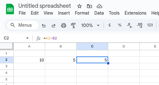
In the example below, we've got the number '10' in cell A2 and the number '5' in cell B2. To subtract the number '5' from the number '10' you would do the following.
How to subtract from one cell:
Click on cell C2, which is the cell where you'll enter the formula
Enter the formula =A2-B2
or
Click on cell C2
Type the equals sign '='
Click on Cell A2
Type the minus sign '-'
Click on Cell B2
Press the return key
The answer in cell C2 should be 5.
Subtracting from a range of cells in Google Sheets
You can also subtract from a range of cells. Using a range of cells in your formula will make it much quicker than subtracting from each cell individually.
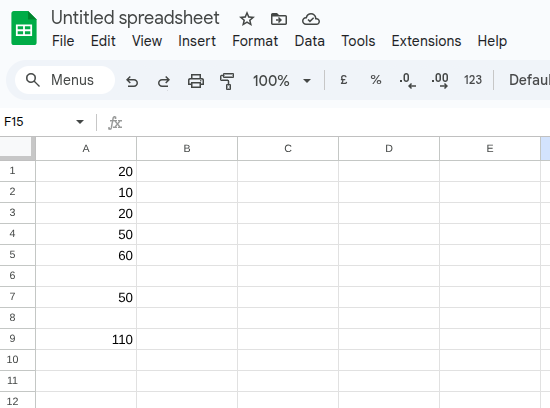
Below, you have numbers in cells A1 to A5, and you want to subtract the total of these numbers from cell A7. You'll be entering the formula in cell A9.
How to subtract from a range of cells:
Click on cell A9
Enter the formula =sum(A1:A5)-A7
This formula has added the numbers in cells A1 to A5, which is '160' and then subtracted the number '50' from cell A7. This should bring back the result of '110'.
Subtracting one range of cells from another range of cells
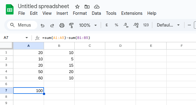
You can also subtract a range of cells from another range of cells. In the following example, we have a range of numbers in cells A1 to A5 and we want to subtract that total from cells B1 to B5. The formula is entered into cell A7.
How to subtract one range from another range:
Click on Cell A7
Enter the formula =sum(A1:A5)-sum(B1:B5)
This formula adds the numbers in cells A1 to A5 and then subtracts the sum of B1 to B5. You should get the answer of 100.
Subtracting one formula from another formula
The examples we've looked at so far all work fine, as they bring back the correct result. However, in practical terms, it would not make much sense using such formulas.
It would most likely be the case that you would regularly need to subtract the numbers in column A from the numbers in column B. So it would make sense to total these numbers together using a formula. You can then create a separate formula to do the subtraction.
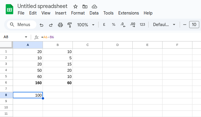
Using the method above provides you with more information about the total of Cells A1 to A5 and cells B1 to B5 without having to do a manual calculation in your head. You can then perform a separate calculation in cell A8 for the subtraction.
The formulas used:
In cell A6 =sum(a1:a5)
In cell B6 =sum(b1:b5)
In cell A8 =A6-B6
This provides the same answer of 100, but it also uses formulas to total the range of cells used in the calculation. This makes it much easier to read a spreadsheet and get the information you need.
What next?
You’ve just read ‘How to subtract numbers in Google Sheets’, use the links below to go to the next section or go back to the Google Sheets Hub.
Understanding the basics of Spreadsheets
How to add numbers in Google Sheets
How to subtract numbers in Google Sheets
How to multiply numbers in Google Sheets

Google Sheets - Understanding the basics of spreadsheets
Google Sheets is a spreadsheet program that you access from the internet. All of the work you do with Google Sheets is done online. This has many advantages because it means you don't need to worry about making sure you have the latest version.
It also means you can share worksheets with your colleagues, so you can all work on one spreadsheet at the same time. When Google Sheets originally launched, it was the only spreadsheet program, which truly offered online collaboration. Since then, Microsoft has also launched an online version of Excel, which is the most well known and used spreadsheet program in the world.
The great thing about Google Sheets is that it's free to use, which is great when you consider Excel can cost a lot of money. Especially if you have to buy many licenses to cover your users.
This page explains the absolute basics of using Google Sheets. It's worth pointing out spreadsheets, in general, whether you're using Google Sheets or Excel, work on the same principle. So if you already have an understanding of spreadsheets the information covered may already be familiar. However, there are some differences with Google Sheets, so it's still worth a read.
What is a spreadsheet?
A spreadsheet is a powerful application and is used in every business you can think of around the world. Whether that business has one employee or is a multinational employing thousands they'll be using a spreadsheet.
The primary goal of a spreadsheet is to organise, analyse and calculate data. However, the spreadsheet has become so commonplace in the working environment that it's usually used for many other tasks. For example, a lot of businesses use a spreadsheet to store data. This is fine, but it's not perfect because to store data, you should really be using a database.
A spreadsheet isn't just limited to the business sector, as it can be used for personal use as well. For example, you may want to create a spreadsheet to help with your household budget. A spreadsheet is perfect for this type of task.
Understanding the basics of a spreadsheet
To be confident using a spreadsheet, you must understand the basic principles. When you are new to using a spreadsheet, it can feel daunting, but once you’ve mastered the basics, you’ll feel more confident using the more advanced features.
Cells
When you first open a spreadsheet, you’ll be presented with what looks like a large blank white space. However, you will also notice lines going horizontally and vertically across the page. These lines help to separate the cells, so it’s easy to navigate and locate a specific cell.
Each cell has its own unique reference, which is extremely useful and important to understand. The reference of the first cell in a spreadsheet is A1. This is because it’s located in column A, Row 1. In the image below I’ve added the figure 150 to cell D4, which you can easily locate by finding column D, then Row 4.
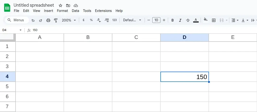
Cell D4 contains the value 150
It’s important to understand how cells work, as they are used to enter all the data into a spreadsheet. Each cell can contain separate data, whether it’s alpha or numeric.
Cell references are important as you’ll use these to do simple math or more complicated data analysis.
A range of cells
A range of cells refers to a group of cells, which you’ll use a lot more when using a spreadsheet over time. For example, you may want to subtract numbers contained in several cells from the number in another cell or a range of cells.
In the image below you can see data in cells A1, A2, A3, A4 and A6. Rather than referencing cells A1,A2,A3,A4 to group those cells. When using a spreadsheet, you would reference this range of cells as A1:A4. A1 is the first cell, and A4 is the last, and the colon acts as the word “to” when referring to a range of cells in a spreadsheet. In other words, cells A1 to A4 are A1:A4.
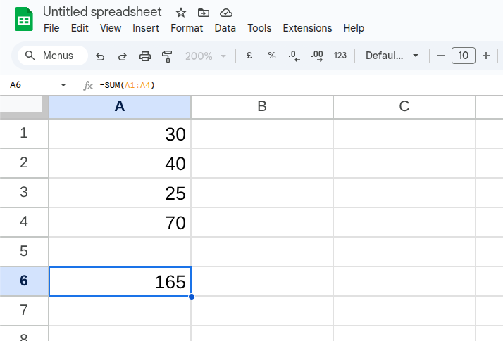
The Formula bar shows =SUM(A1:A4)
The numbers in A1:A4 are fixed values. What I mean by this is that I entered the number 30 into A1, 40 into A2, 25 into A3 and 70 into A4.
In cell A6, you may see the number 165, but this isn’t a number I entered manually. Instead, it’s a formula using the range of cells we’ve mentioned to calculate the total. You can see this in the Formula Bar, which is located above the spreadsheet grid.
In the formula bar, you’ll see I’ve entered the following formula:
=sum(A1:A4)
What next?
You’ve just read ‘Understanding the basics of spreadsheets’, use the links below to go to the next section or go back to the Google Sheets Hub.
Understanding the basics of Spreadsheets
How to add numbers in Google Sheets
How to subtract numbers in Google Sheets
How to multiply numbers in Google Sheets
How to add numbers in Google Sheets
Adding numbers together in Google Sheets is easy to do. Spreadsheets are extremely powerful programs and learning how to do basic calculations is important. Once you've mastered how to do the basics you'll feel more confident using a spreadsheet program such as Google Sheets. Let's take a look at how to add numbers in Google Sheets.
There are two ways to add numbers together in Google Sheets
The great thing about spreadsheets is there isn't necessarily just one way of working. Everyone calculates differently and as long as you get the right calculation at the end it does not matter too much about the calculation you used.
However, some ways of calculating are more efficient than others. Google Sheets will let you calculate numbers in whatever way you feel is right. Providing the formula is correct it will bring back the correct result.
There are two ways of adding numbers together in Google Sheets and we'll take a look at both of them here. The way you decide to add numbers together is a personal preference, but you'll soon see how one way is more efficient than the other.
Adding cells together individually
This is the most basic way of adding cells together in Excel. It is usually only ideal to add numbers together this way if you don't have many cells to add up.
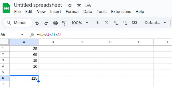
Above, we have numbers in rows one to four, and we want to add these numbers together. We'll use cell A6 for the formula.
In cell A6, you would type the following formula:
=a1+a2+a3+a4
You can either type the formula or after typing the '=' sign you could click on cell A1 then press '+' then click cell A2 then '+' and so on. This will make it quicker than typing the whole formula.
Adding cells together using =sum
As we've seen, you can add cells together in Google Sheets individually. However, imagine how long this would take if you had many cells included in the formula.
The best way to add numbers in a spreadsheet is to use SUM. Using SUM provides a much quicker way of doing calculations in a spreadsheet.
Whenever you wish to perform a calculation in a spreadsheet, you always start with the equals sign. If you just typed sum (A1:A12) into a cell, the spreadsheet will assume you want to add this as fixed text, and no calculation will take place.
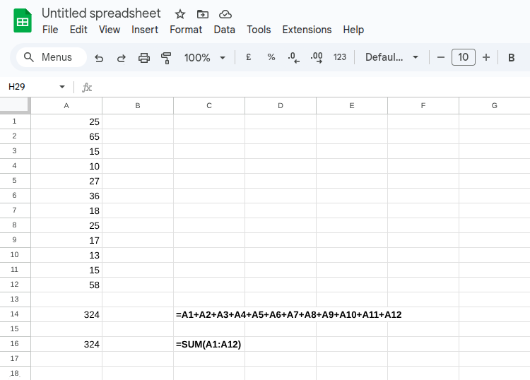
In the spreadsheet above, you can see figures in cells A1 to A12. In cells A14 and A16, you can see the figure 324, which is all the numbers added together in A1:A12. You’ll notice I’ve shown the sum used for both A14 and A16 in both C14 and C16. You can clearly see it’s much quicker to use the =sum formula.
Google Sheets can predict the formula for you
You may have noticed when typing the formulas earlier into Google Sheets that it automatically recommends the formula you may want to use. This is really handy because it means you don't need to do the formula yourself. Although this is handy, it may not always be the formula you want.
However, it's worth pointing out that sometimes Google Sheets will provide you with formulas that you may want to use. To use these, when you start typing the formula and the dialogue box appears with recommendations. You simply tab down to the recommended formula you want to use and hit the return key.
What next?
You’ve just read ‘How to add numbers in Google Sheets’, use the links below to go to the next section or go back to the Google Sheets Hub.
Understanding the basics of Spreadsheets
How to add numbers in Google Sheets
How to subtract numbers in Google Sheets
How to multiply numbers in Google Sheets